Introduction

Newcomb’s paradox is a famous thought experiment in decision theory, where two ways of thinking that seem equally logical lead to completely opposite conclusions. It is often posed as an opposition between two principles for making decisions: Evidential Decision Theory (EDT) and Causal Decision Theory (CDT), with EDT deriving one-boxing and CDT deriving two-boxing. Although I am a supporter of one-boxing, I actually do not think EDT makes sense, for reasons I will not elaborate on in detail here. Instead of justifying one-boxing from an EDT perspective, I will be digging into the core and hidden assumptions we typically make when we are thinking about a decision, with the help of formalized CDT. I will then show that a naive application of CDT undermines the fundamental setup of Newcomb’s problem, and that a correct application of causal-based reasoning actually justifies one-boxing.

Problem Setup

Imagine there is the Predictor, perhaps a superintelligent AI, who knows you better than yourself. The Predictor can make very good predictions about your decision. As a simplification, let’s just assume the Predictor is infallible for now (accuracy does not matter much for the arguments below).

You walk into a room. In front of you are two boxes, already set up by the Predictor:

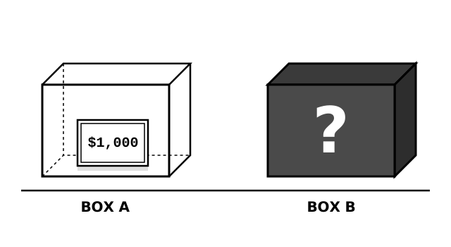A visual representation of Newcomb's Problem.

• Box A is transparent, and you can see that it always contains $1,000 dollars.
• Box B is opaque and contains either $1,000,000 or nothing.

Your goal is, of course, to gain as much money as possible, and you are given two choices:

1. Take only Box B
2. Take both boxes

The actual content of Box B is already set before you make your choice, and the Predictor had filled it according to the following rule:

• If the Predictor predicted that you would take only Box B, it placed $1,000,000 inside.
• If the Predictor predicted that you would take both boxes, it left Box B empty.

Now, standing in front of the boxes, you know the rules, and you know how good the predictor is. The money is already set in the boxes, not to be altered by any mechanism.

Do you take both boxes, or only Box B?

There are two main camps on this problem, corresponding to the two choices available.

Two-boxers’ Argument

Two-boxers’ argument goes like this:

1. The money is already set in the boxes, not to be altered by any mechanism.
2. Therefore, if I take both boxes, I will always end up with \$1,000 more than if I take only Box B. In detail:
   1. If there is \$1,000,000 in Box B, taking both boxes yields \$1,001,000, while taking only Box B yields \$1,000,000.
   2. If there is nothing in Box B, taking both boxes yields \$1,000, while taking only Box B yields \$0.
3. In conclusion, taking both boxes is superior.

Appealing right? Take a moment to ponder this, see if you can find any flaw in this argument. When you are ready, move on to the next section.

One-boxers’ Argument

One-boxers’ argument, in contrast, goes like this:

1. If I choose to take only Box B, the Predictor would have predicted it, so I get the \$1,000,000.
2. If I choose to take both boxes, the Predictor would have predicted it, so I get \$1,000.
3. In conclusion, taking only Box B is superior.

Who’s the Winner?

Before we drown ourselves in endless debates on whose intuition is correct, I think it is important to know who actually wins in this game.

Suppose the AI is really infallible as the problem stated, the two-boxers would be predicted to take both boxes, and thus end up with only \$1,000. In contrast, the one-boxers would be predicted to take only Box B, and thus end up with \$1,000,000. Since the common goal is to gain as much money as possible, the one-boxers are clearly the winners.

A hidden but important assumption I am making here is that humans are just physical systems. In principle, with enough information gathered by the Predictor, it would be able to predict a person’s precise judgment and decision. There is no mysterious “libertarian free will” that allows a person to break away from the causal structure of the person, which the Predictor relies on to make reliable predictions.

Under this assumption, the analysis above holds and the two-boxers lose. There is no room for debates here. The rest of the discussion is just to explain why two-boxing, although reasonable, is wrong in this particular setting.

A Quick Comparison

One general rule I’ve found dealing with mathematical or logical problems is that the more accurate assumptions you make of the problem, the better you would be able to solve it. On the other hand, the worse your assumptions align with the problem, the more you deviate from the optimal solution.

If you compare the two arguments above, you should be able to see that

1. Two-boxers and one-boxers both made use of the game rule about boxes and the money placed in it.
2. However, only the one-boxers used the fact that the Predictor is a good predictor. The two boxers’ argument ignores this fact.

Therefore, it is not surprising to me that one-boxers win. Two-boxers’ argument simply does not take advantage of the assumptions you are allowed to make in this problem.

Of course, you might still find this unsatisfying, so read on. It gets more interesting when we dig deeper into why most people find two-boxing intuitive. To analyze this, I think it would be helpful to introduce some basics of Causal Decision Theory, with the visual help from Bayesian networks, as nicely summarized in Judea Pearl’s Causality [1]. It formally describes a process of making decisions, that forces us to be explicit about the assumptions we make.

Causal Decision Theory

To understand what making a decision means in a causal model, let’s first consider a simple example taken from Causality [1].

Here is a Bayesian network representing the causal relationships between the variables related to the pavement being slippery:

    graph TD
    Season((Season)) --> Sprinkler((Sprinkler))
    Season((Season)) --> Rain((Rain))
    Sprinkler((Sprinkler)) --> Wet((Wet))
    Rain((Rain)) --> Wet((Wet))
    Wet --> Slippery((Slippery))
  

In plain words, the Bayesian network models these causal relationships:

1. Season influences people’s decision to turn the sprinkler on or off.
2. Season influences the chance of rain.
3. Both the sprinkler and the rain can make the pavement wet.
4. The pavement being wet makes it slippery.

Now, suppose a curious agent would like to study exactly how the sprinkler affect the pavement’s slipperiness (I will use the word agent instead of person from now on since this analysis applies to any system that makes decisions and takes actions). The agent would intervene on the sprinkler, i.e., forcefully turning it on or off, ignoring the usual influence from the season. Then, the agent would be able to observe exactly how the slipperiness changes following from their intervention on the sprinkler. This can be represented by the modified network, with a double circle representing the intervention or action of an agent:

    graph TD
    Season((Season)) --> Rain((Rain))
    Sprinkler(((Sprinkler))) --> Wet((Wet))
    Rain((Rain)) --> Wet((Wet))
    Wet --> Slippery((Slippery))
  

This is the basic framework of Causal Decision Theory. The action to be evaluated is the node with double circle, representing a free variable that can be controlled by an agent. One can understand this intuitively: when the agent deliberately chooses an action, the causal structure of the world has been modified so that, the sprinkler, instead of following its usual, observed causal relationship, is now attached to the agent’s will. To experiment or optimize a decision, we can imagine setting the action node to all possible values, calculate how the rest of the variables change accordingly, and compare the expected outcome of interest. Then, we choose the action that yields the best expected outcome. For example, to maximize the expected slipperiness of the pavement, the agent would discover that turning the sprinkler on yields higher expected slipperiness than turning it off. Turning it on is then the optimal choice relative to this goal.

I’ll point out a few observations that relate to our discussion later. It will be the key to see why a naive application of Causal Decision Theory fails on Newcomb’s Problem. First, the action node, which represent the agent’s choice, is assumed to be independent of any upstream causes in the first graph. Second, it is also worth mentioning that the agent is not explicitly modeled in the graph, but only the final action of the agent is included as the special action node. This makes sense due to the first assumption on independence.

Causal Analysis of Newcomb’s Problem

Following our current understanding of human mind, which can be thought of as a complex machine operating according to the laws of physics, I think we can model the Newcomb’s Problem very roughly like this:

    graph TD
    X(( X )) --> B((Box B))
    X --> D(("Decision"))
    D --> M((Money))
    B --> M
  

Here, $X$ represents whatever factor that determines the agent’s choice, it may include the internal states and tendencies of the agent, such as genetics, education, personality, temporary mood, or even any environmental factors that conditions the agent’s choice. The final decision of the agent (drawn as the Decision node) thus follows from $X$, according to the laws of physics. To make predictions about the decision, the Predictor must have gathered information about $X$, and filled the boxes accordingly. The link from $X$ to Box B in the graph models how Predictor gather the information and make prediction to decide the content of Box B. Finally, the money the agent receives (drawn as the Money node) is determined by both the content of the boxes and the agent’s decision. The expected money is the target we are interested in maximizing.

Applying Causal Decision Theory

To apply Causal Decision Theory to the Newcomb’s problem, one might be tempted to modify the graph above in the same way as we did in the sprinkler example, i.e.:

    graph TD
    X(( X )) --> B((Box B))
    D((("Decision"))) --> M((Money))
    B --> M
  

We have severed the link from $X$ to the final decision made by the agent, treating the decision as a variable we can set freely and evaluate the outcome.

However, this is exactly where the problem lies. If the agent’s decision does not follow from $X$ according to laws of physics, how does the agent even make choices? The agent themselves must be part of the world, implemented by physical matters, ran by physical laws, right? If we were to detach the decision from its own internal states and process, who is determining the decision? This seems to be sneaking in a kind of uncaused cause, a ghost in the machine, or an invisible homunculus “actually” making the decision, ignoring all previous causes. This simply does not make sense according to our modern understanding of nature, and contradicts research findings in biology and neuroscience, where in most if not all cases, the human mind does behave like a law-following physical system. Furthermore, if the decision were really free from previous causes, there would be no causal relation nor correlation that the Predictor can follow to make reliable predictions. It breaks the whole predictability assumption of Newcomb’s problem.

In the sprinkler example, we can sever the sprinkler’s connection to season and transform it into an action node, because the agent is a new causal upstream that determines the sprinkler’s state, and the whole causal chain implementing the agent is assumed to be independent of the rest of the graph, thus collapsing into a single action node.

However, in the Newcomb’s problem, the agent’s internal state $X$ has become an upstream variable that determines both the agent’s decision and the content of the box. We can no longer just collapse it into a single action node nor disconnect it from the final decision.

Suppose we really follow through on this faulty application of CDT, we would perform the following reasoning and falsely concluding that two-boxing is superior:

1. The content of box B is determined by its own isolated causal chain, which can be simplified as having probability $p$ of containing a million dollars, and $1-p$ of containing nothing.
2. The expected return of the two choices are:
   1. One-boxing: $p \times 1,000,000 + (1-p) \times 0$
   2. Two-boxing: $p \times 1,001,000 + (1-p) \times 1,000$
3. For any $p$ between 0 and 1, the multiplier of $p$ and $(1-p)$ are both larger in the two-boxing case. (This is essentially the strategic dominance argument.)
4. Therefore, the expected return of two-boxing is always greater than that of one-boxing.

Although the whole analysis is correct following from the graph, the graph itself is constructed incorrectly. It has broken the causal relationship that is crucial to both the Predictor’s prediction and the agent’s decision.

Applying Causal Decision Theory (Correctly)

Newcomb’s problem is often posed as a rivalry between Causal Decision Theory and Evidential Decision Theory (EDT), each deriving two-boxing and one-boxing respectively. Despite the fact that EDT derives one-boxing, I am generally skeptical of EDT. EDT derives obviously wrong conclusions in some cases such as the smoking lesion problem, and seems to have a confused stance on whether the action is caused by upstream factors or by an agent capable of total control over its action. To focus on the topic, I’ll leave EDT aside.

What I really want to do here, is to show that making decisions using a “causal” mindset still make sense, even in weird cases like Newcomb’s problem. We just have to be careful over what we are “choosing” and make sure that our causal model aligns with how reality works.

Instead of thinking that we are choosing for the final action of taking boxes, we can think of choosing to be a one-boxer or two-boxer, which is defined by the collection of internal states or factors that leads to the final action. Under this framework, we can create such a causal model:

    graph TD
    T(((Type))) --> B((Box B))
    T --> D(("Decision"))
    D --> M((Money))
    B --> M
  

1. The “Type” are the collection of factors or states (that may not necessarily be part of “us” in common sense) that determine “who we are” at the beginning of the game. Notice that Type, not the Decision, is now the double-circled node. We are now imagining we can set these factors to change “who we are” and thus affecting the decision we make.
2. The “Decision” is our choice of taking one or two boxes, it follows from our “Type” which determines the reasoning process and thus the final decision.
3. The “Box B” is the content of the box, filled by the Predictor using information about our “Type”.
4. The “Money” is the payoff, it follows from the “Decision” and the “Box B”.

Notice now that the problems we see in the previous section have been solved. This model successfully preserves the causal relationship from the agent’s type to their decision, as well as to the Predictor’s prediction. Using this new model, we can then derive one-boxing from a purely causal framework. To reveal more insights, I am also allowing the Predictor to be fallible in this analysis.

1. Assume that the Predictor have a probability $p$ of being correct regardless of our type.
2. The expected return of the two choices are:
   1. One-boxing: $p \times 1,000,000 + (1-p) \times 0$
   2. Two-boxing: $p \times 1,000 + (1-p) \times 1,001,000$
3. With some basic algebra, we can derive that one boxing is better in expectation if and only if $p > 0.5005$.

Notice that $p = 0.5$ is the accuracy the Predictor gets when it simply flips coins to make predictions without using any information about the person. Therefore, we can roughly say that one-boxing is better whenever the Predictor is non-trivially good at prediction. Two-boxing is better when the Predictor is close to random guessing, which becomes close to the model in the previous section, where the decision is incorrectly assumed to be independent of the prediction.

Can We Really Choose Our Type?

When I shifted the intervention from the Decision node to the Type node, I seemed to have silently sneaked in a generalization over what can be intervened on. In contrast, the intervention happens on the final action of an agent in typical CDT setups. This naturally invites a question: Can we really “choose” our type? Is this generalization justified?

Interestingly, the same question can be asked for typical CDT setups: Can we really “choose” our action? If we commit to the physicalism I had been holding throughout this analysis, that would mean all the actions we performed are ultimately consequences of some upstream cause. If so, does arguing over decisions even make sense?

I think a thorough discussion of this would easily expand into a broader discussion on compatibilism, so maybe I will just keep it short here. I think CDT does not really assume the intervention to be “free” in the libertarian free-will sense; it just has to be “free in our limited model” — a node we are intervening on shall not also be a downstream effect of another node in our model, even if it is ultimately a downstream effect under a larger model. The intervention node in the causal graph can be thought of as simply an injection point in our model for us to plug in an initial condition, play through the modeled dynamics, predict the consequence, which allows us to evaluate our decision (or more generally, to evaluate the factors we plugged in). In other words, it is an evaluative device that works as long as it models the world correctly. A superior decision is superior regardless of whether we are free.

A discussion on what decision should be made still makes sense, even if the decision were already determined at the moment you walk into the room. Similarly, an evaluation over what type of person we should be is still meaningful, even if you were determined to be a one-boxer after reading this article. Let this be the upstream cause!

.  .  .

Summarizing Newcomb’s Problem

In summary, Causal Decision Theory typically assume the action to be coming from an independent causal source, i.e., the agent, and it is mostly correct in daily life, where our internal state is sufficiently independent of the immediate environment. The two-boxing argument seems so intuitive at first glance exactly because it does work most of the time in practice. However, in some cases, such as Newcomb’s problem, this assumption of independence is broken, making this intuition misleading. Luckily, it seems we can still correctly apply Causal Decision Theory by thinking carefully about what we are choosing and make sure we are not breaking the causal structure of the problem.

As long as you do not believe an agent like us can somehow make decisions in an uncaused fashion, I think the analysis above should be a solid answer to why two-boxing is wrong.

References

- J. Pearl, Causality: Models, Reasoning, and Inference (2000). Cambridge University Press.